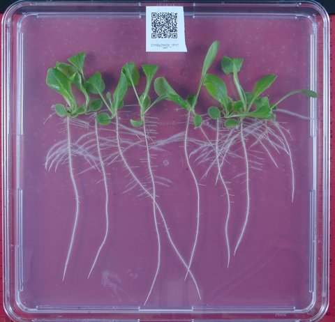
RootSegmenter labels plant roots in images. A labeler corrects the program's output, the corrections train a neural network (Convolutional U-Net), and the network becomes the starting point for the next image. Twelve labeled images were enough to cut labeling time by more than half and raise label quality from roughly .93 Dice to roughly .98. The two best existing tools in the field score between .45 and .74 on the same datasets.
Run the tool yourself on one of these plates, or keep reading to see how it works.
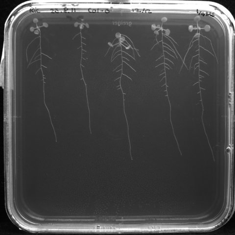
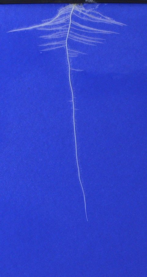
These pages are the full program. Every stage runs live on your machine, and you can change any setting and see the result. Nothing is uploaded anywhere.
How it works
The program works in nine stages. The user steps through them, adjusting settings and watching the labels update, and can return to any previous stage using undo.
Start from the neural network
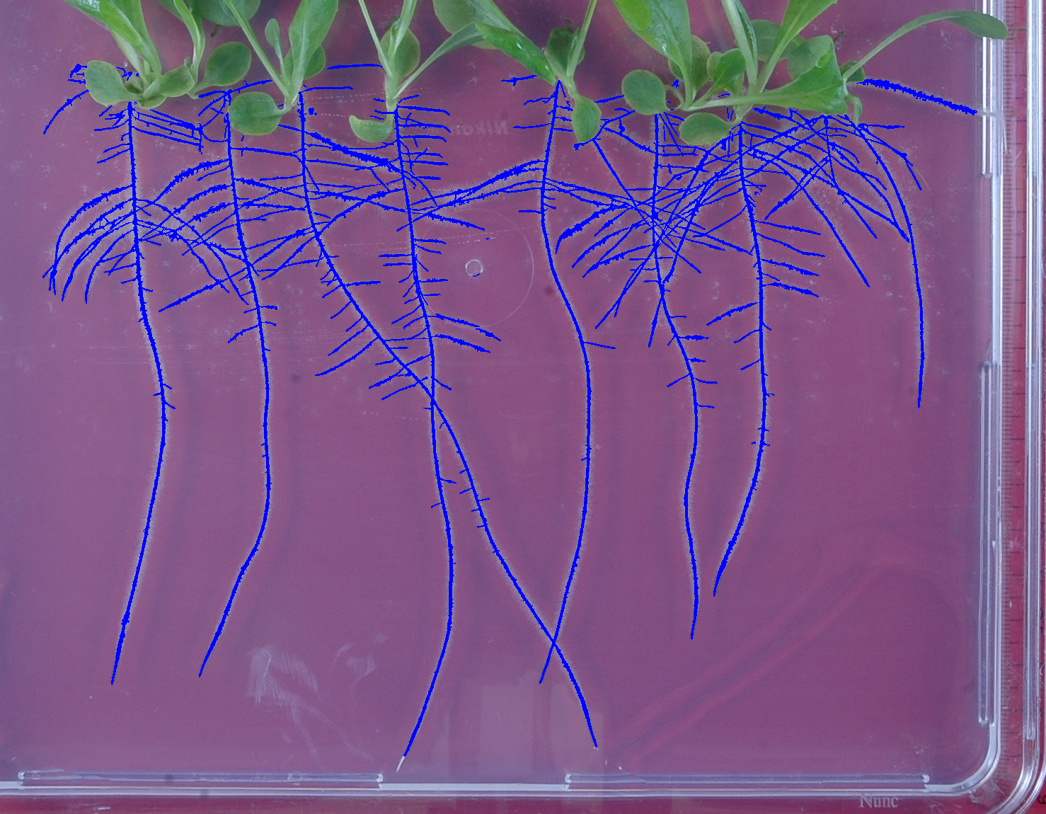
This is the network's output on the lettuce plate, with no human input. Drag the slider to compare it with the raw image. The network was trained on 4 labeled images, with 2 validation labels.
Network Performance
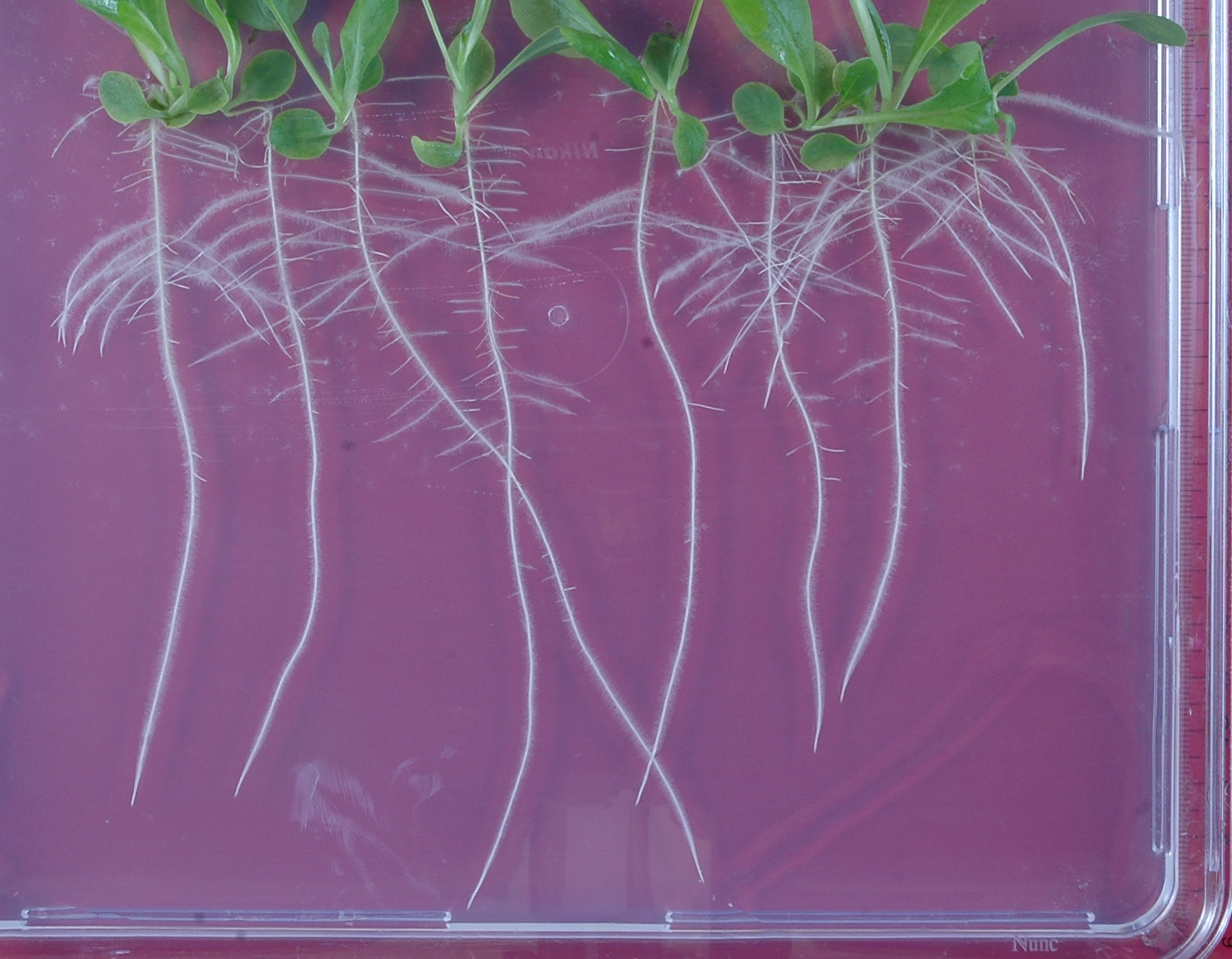
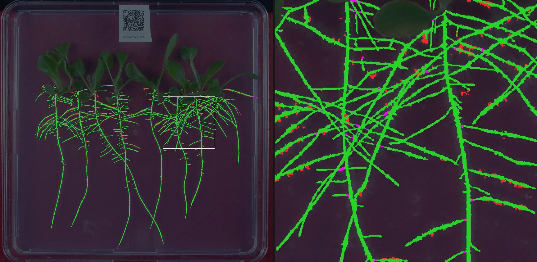
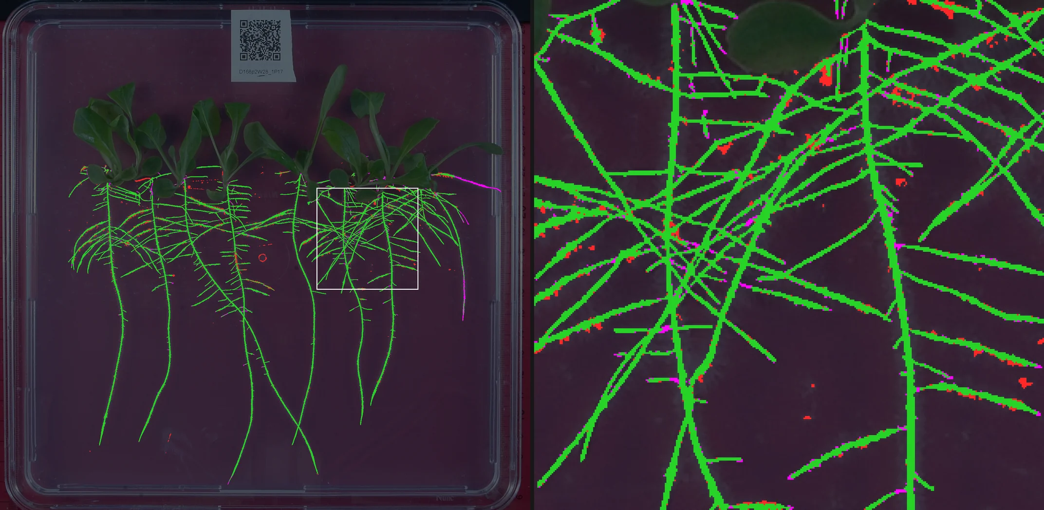
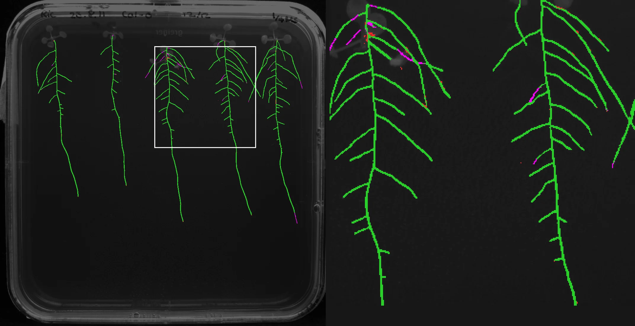
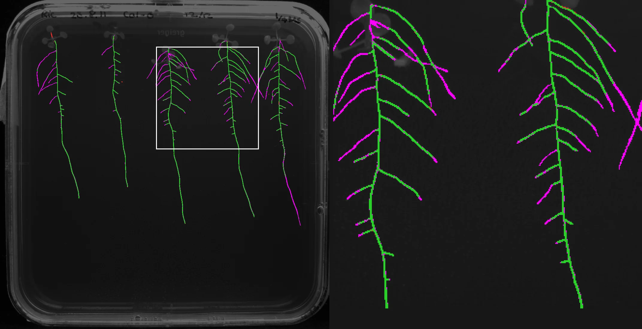
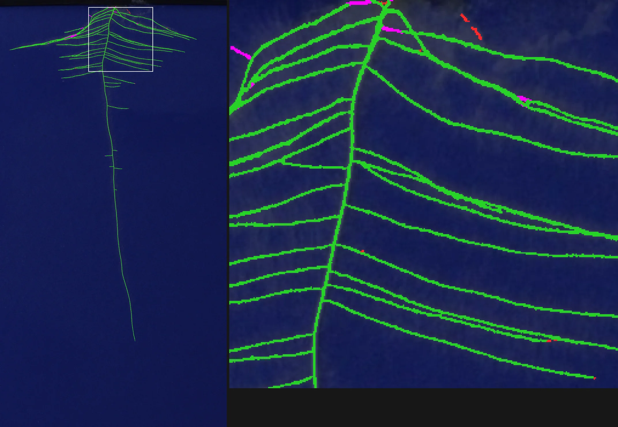
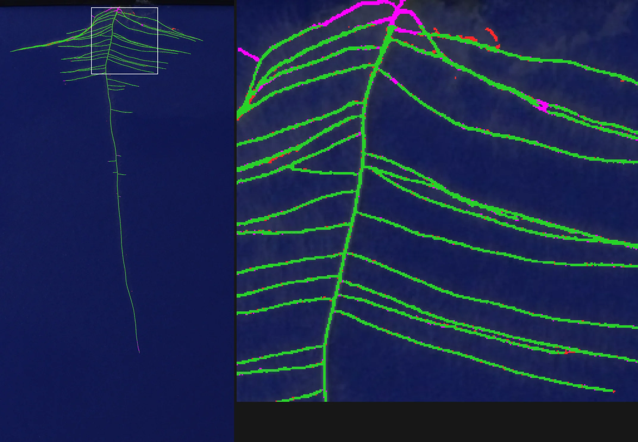
Each image compares a network's labels with the ground truth on the same plate. The left side is the whole plate. The right side zooms into the white box, the part of the plate with the most roots.
The paper network is the most trained network from the paper for that species. The 1-plate network was trained on a single plate for 2,000 epochs. Training on a single image for 2,000 epochs without a validation set seems to be safe in general, because the network is resistant to overfitting and followed a consistent validation loss curve when tested across all 3 datasets.
- Green: network and ground truth
- Red: network only
- Magenta: ground truth only
- Dimmed plate: neither
Two-click root tracing
On the manual correction stage, click one end of an unlabeled root and then the other, and the program traces the root between the two clicks. The trace follows the root's curves and stays on it where other roots cross.
Gaussian filter
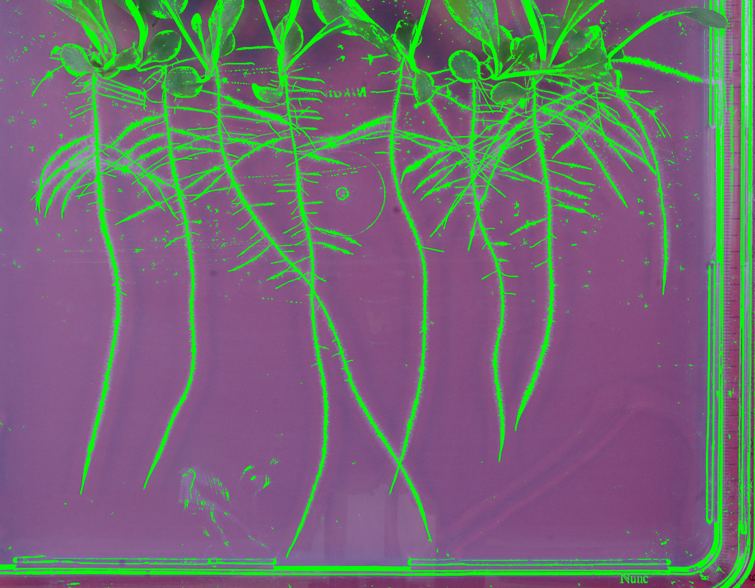
The Gaussian filter selects pixels brighter than their neighbours. Its purpose is to produce a mask of candidate pixels, so false positives are fine as long as there are no false negatives. It is the first stage of the classical pipeline, shown here on the lettuce plate. Drag the slider to compare it with the raw image.
Label cropping
Click to place the corners of a polygon around the growth area. Enter keeps the inside, and Shift+Enter keeps the outside.
Texture matcher
Left click on background and right click on roots to give examples. An SVM uses them to classify every patch. The black pixels are incorrect labels the texture matcher removed as background. The examples are saved and loaded for future images from the same dataset.
Connect separated roots
The Gaussian filter and edge finder tend to drop pixels where a bright root crosses a darker one. This stage rejoins them. Newly connected pixels are shown in orange.
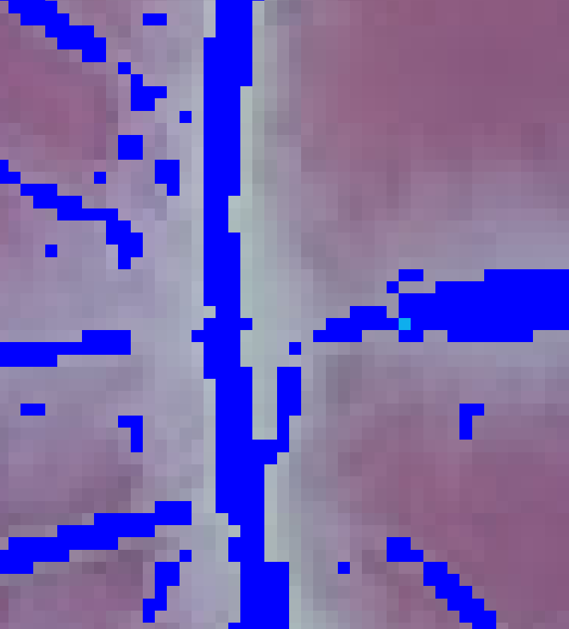 Before
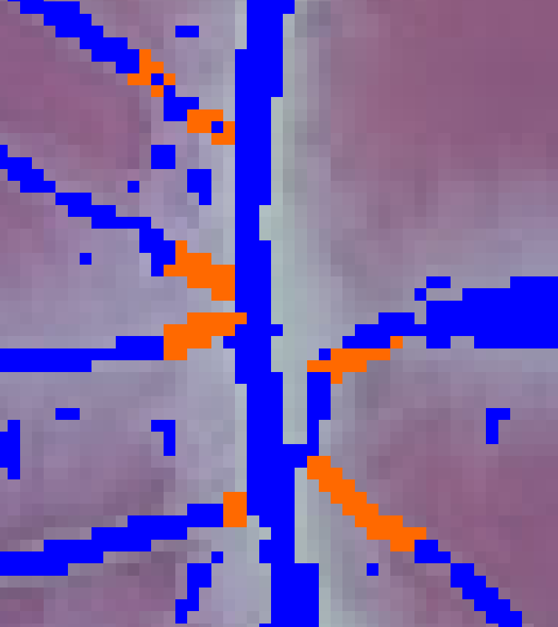 After
AfterResults
These are the results from the paper. Every column is driven by a human labeler except the two marked Auto, which show the network running with no human input at all. Neural Net 6 and Neural Net 12 mean the network was trained on that many labeled images.
Average Dice coefficient, where higher is better:
| Dataset | RootNav | saRIA | Project | Neural Net 6 | Neural Net 12 | Neural Net 6 Auto | Neural Net 12 Auto |
|---|---|---|---|---|---|---|---|
| Main | N/A | .6584 | .9313 | N/A | .9769 | N/A | .9702 |
| Arabidopsis | .6619 | .7350 | .9420 | .9721 | .9893 | .9548 | .9829 |
| Rapeseed | .6279 | .4539 | .9272 | .9529 | .9826 | .9407 | .9780 |
Average seconds to label one image, where lower is better:
| Dataset | RootNav | saRIA | Project | Neural Net 6 | Neural Net 12 |
|---|---|---|---|---|---|
| Main | N/A | 199 | 865 | N/A | 403 |
| Arabidopsis | 379 | 164 | 245 | 148 | 108 |
| Rapeseed | 487 | 106 | 510 | 197 | 145 |
The accuracy gap is large. The difference between .93 and the .45 to .74 range is the difference between labels that can be published and labels that have to be discarded. The network paid for itself after twelve labeled images. It cut labeling time by at least a factor of two, and raised accuracy at the same time.
There were no quality ground truths for any of the datasets, so new ones had to be produced with this program. A significant portion of the network's predictions were kept in the ground truths, so it is likely the neural networks obtained a moderately higher score than they should have. That bias only affects the comparison between the project's own columns. It cannot account for the gap against saRIA and RootNav. The full evaluation is in the paper.
How this page works
The desktop program is written in Python and C++. For this page, all of it was ported to a single C++ library and compiled to WebAssembly, so it runs in the browser at close to native speed. The network runs through ONNX Runtime Web.
The port was checked against the original program instead of being trusted. Every stage, every correction tool and the undo history were tested to produce output identical to the desktop program, pixel for pixel, on all three plates. Additionally, every test was checked by deliberately breaking the code it covers and confirming the test fails.